Most of our customers who use our Microsoft Excel add-ins CDXZipStream and CDXStreamer for address and location analysis, are working with a lot of data in an Excel worksheet. And if CDXZipStream or CDXStreamer are used to provide additional information for each point of data, it can be quite a task managing and analyzing all the results. Here are some tips on how to approach data in a large Excel worksheet, particularly on how to find the data you need within a large data set.
First, if the data returned from the add-in is in formula form, get rid of the formulas by copying them to values. Just select the area containing the formulas, and use the paste special option to paste values only. The formulas will be replaced with their values; if a worksheet contains a lot of formulas, this will significantly speed up subsequent worksheet processing you’ll be doing later. As an alternative, you can use the “Set Array to Values” option in the address verification function of CDXStreamer. (You can also check out the navigation shortcuts described in our blog article 5 Handy Tips all Excel User Should Know, which can help you move around and select large data sets.)
But how do you find just the data you need, in a very large worksheet? Here are three ways available to do this efficiently and easily through Excel:
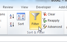
FILTERING: This is Excel’s version of sorting on steroids. The filter option allows you to look for items in a list based on lots of different criteria (that apply to both text and numeric values), and then hides the rows that don’t apply. Select a cell within your data, and in Excel 2007 and up, from the Data tab on the ribbon, click the filter icon:

You’ll notice that drop-down arrows are now visible next to each column of data. (You should make sure to label each column, so the first row of data is also part of the filtering process.) Then click on the arrow in the column you’d like to filter, and based on the type of data present, you’ll be presented with text or numeric filter options. You’ll also be able to do straight-on sorting as well from here, but we’ll focus here on the filter functions. For instance, if we just used CDXZipStream to calculate distances from a target destination, we can find all locations within a 50 mile radius by selecting the following options in the custom filter dialog:

A nice bonus is if you copy and paste the filtered data to another worksheet, the hidden rows are not included. To remove the filter and show all rows of data, just click on the filter icon again. For more information on filtering in Excel, please refer to the following Microsoft article: Filter Data in a Range or Table.
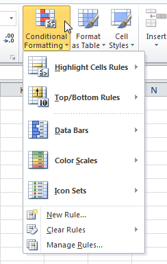
CONDITIONAL FORMATTING: You can change the font, fill, and border colors and formatting depending upon the cell value. From the Home tab, click on Conditional Formatting:

Using the example above, click on Highlight Cells Rules, and specify formatting for values less than 50:

For more information, check out the Microsoft article Add, change, find, or clear conditional formats.
You can also combine conditional formatting with filtering, by using the “sort by color” option available in each column drop-down menu. Please refer to the article Filter by cell formatting.
VLOOKUP/HLOOKUP: Excel VLOOKUP or HLOOKUP are great worksheet functions that can link tables together when they have a common column or row of data. For this example we’ll use VLOOKUP, which is applied to column-oriented data. Let’s say we have a list of routes which have all been optimized using CDXZipStream; we would like to list all the destinations with their contact telephone numbers, but the optimization process has changed their order from their original list. To find the telephone numbers in the original list associated with each destination, we create another column with the formula:
=VLOOKUP( LOOKUP_VALUE, TABLE_ARRAY,COL_INDEX,[RANGE_LOOKUP]) where
LOOKUP_VALUE = the destination address (in the optimized list)
TABLE_ARRAY = the range of cells that contains the destination addresses and telephone numbers in the original list. The first column of this range should contain the destination addresses.
COL_INDEX = the column number of the TABLE_ARRAY that contains the telephone numbers
RANGE_LOOKUP = A logical value, where “FALSE” indicates an exact match is required
If we use a cell address for the first lookup value, we can copy this formula along all the optimized destinations to find their telephone numbers. Make sure however, that the TABLE_ARRAY range is defined by either a named range, or by using an absolute cell range with dollar signs (e.g $A$1:$D$500).
For a list of optimized destinations in column A, we can search for the corresponding telephone number in the range $H$1:$K$200, where the destination addresses are in column H and the telephone numbers are in column K, with the formula:
=VLOOKUP(A1, $H$1:$K$200,2,FALSE)
Then just copy this all along the list to find all telephone numbers.
For more information, please refer to these articles about VLOOKUP and HLOOKUP.