Our Microsoft Excel add-in for zip code and location analysis, CDXZipStream, can generate zip and postal code lists for various geographies like state, county, and city. But if you need to compare two lists of zip or postal codes from CDXZipstream, you can use the computational power of Excel to do the job. Here’s a couple of different approaches, depending upon the version of Excel you are running:
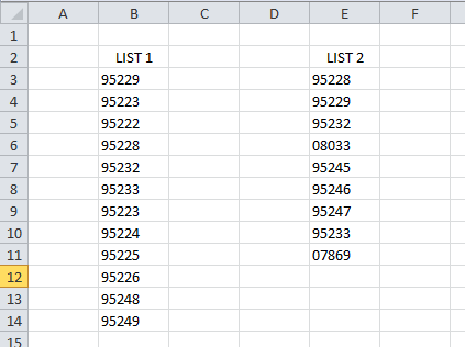
VLOOKUP: The worksheet function VLOOKUP works with Microsoft Excel 2003 and higher versions. For example, let's say we have two zip codes lists like this:

And we want to find which zip codes are in List 1 but not List 2, and vice versa. Just to the right of the first zip code in List 1, in cell C3,we input the formula:
=VLOOKUP(B3,E:E, 1, FALSE)
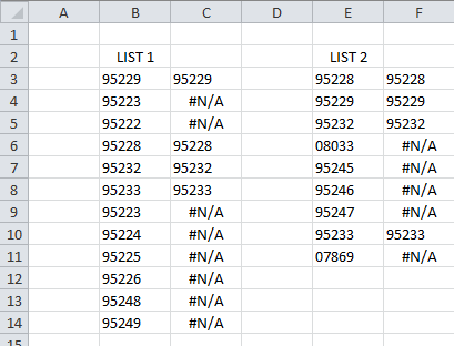
This indicates that we are trying to find the value of cell B3 (ZIP code 95229) in Column E (the location of List 2). If the value is found, the value in the first column (the Zip code) will be returned; if not, “#N/A” is returned. The input value of FALSE indicates an exact match must be made.
We copy this formula all along List 1. We also input a similar formula to the right of List 2 that will search List 1:
=VLOOKUP(E3,B:B, 1, FALSE)
The final result is:

For long lists you may want to use Excel’s sort function to sort these results and more easily identify where the lists are different.
Previously we’ve also shown how you can use VLOOKUP to compare results of zip code radius analysis; for example, identifying the zip codes where two radius areas intersect. Please refer to the blog post ZIP Code Radius Analysis for Multiple Areas for more information.
CONDITIONAL FORMATTING: This method comes to us from Chandoo.org, and can be used in Microsoft Excel 2007 and up:
1. Use the cursor to select the cells in both lists. (After selecting cells in List 1, hold down the CTRL key and select List 2.)
2. From the Home tab, select Conditional Formatting, then Highlight Cells Rules, then Duplicates.
3. You can select to conditionally format unique or duplicate values, and also select color combinations.
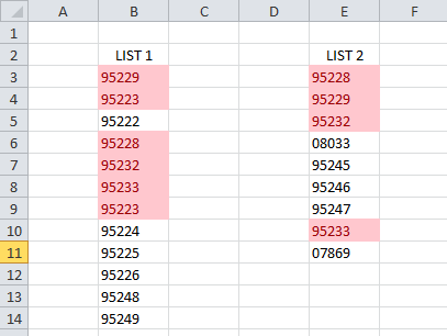
Here is the result, where we highlight duplicate values:

Again, the data can be sorted (based on cell color here) to more easily group and identify differences between the lists.