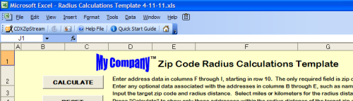
In our last blog we reviewed all the free Microsoft Excel templates we offer for CDXZipStream, that can help you make tasks like route optimization, zip code radius analaysis, and geocoding that much easier. You also have the option to customize the appearance of these templates, particularly to help highlight specific data using Excel built-in functionality. Let’s take a look at the Zip Code Radius Calculations template as an example.
This particular template includes optional data columns B through E that can be used for information like name, telephone number, or any other fields associated with the listed addresses. You can fill in the appropriate field names at the top of the data columns, or if you don’t need to use these columns, just hide them. To hide the columns In Excel 2003, select Format (Column) from the main toolbar, or in Excel 2007 and 2010 use Format (Visibility) from the Home tab. Do not delete these columns, since this will change the location of the input data required for the analysis, and will make the template inoperable.
We also recommend that to ensure you don’t lose any data along the way, you should save the template under a new name both before and after making any major changes.
Now let’s review a few methods to change the display of the template data worksheet. Keep in mind that once these changes are made, you can then copy and paste the results to another blank workbook to permanently save them:
1. Sort - Most users of Microsoft Excel have used the sort function at some point, and it can certainly be used here if you need to sort the input or output data in the worksheet. After pressing “Calculate” in the Zip Code Radius Calculations template, the worksheet will already be autofiltered in order to show the addresses or zip codes that fall within the specified radius distance of the target. But even after autofiltering, the addresses will be shown in the order in which they were entered into the worksheet. If you would like to the addresses in order of their distance to the target zip code, for example, select Data (Sort) from the main toolbar in Excel 2003, or in Excel 2007 and 2010 use Sort from the Data tab. From here you can sort by the appropriate column in either ascending or descending order. For more information about sorting, check out these links for Excel 2003 and Excel 2007-2010.
2. Autofilter – Autofiltering hides any rows that do not meet the filter criteria you specify. For instance, you may want to show only address data for a particular city, zip, or other data field. Since the Zip Code Radius Calculations template automatically autofilters the results based on the distance from the target zip code, you will need to first turn off and then turn on the autofilter if you would like to use this for some other filtering criteria. You can also filter based on two data fields, for example, if you want to show only those addresses within the target radius that are in a single town. To autofilter make sure a cell in the white data area is selected, then select Data (Filter - Autofilter) from the main toolbar in Excel 2003, or in Excel 2007 and 2010 use Filter from the Data tab. For more details about autofiltering, see the following links for Excel 2003 and Excel 2007-2010.
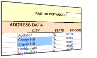
3. Conditional Formatting – This approach usually uses color to highlight data of interest. Just specify the font color, background color, or other format option using similar specifications to autofilter; in this case however, rows are formatted as specified if they meet your criteria, not hidden if they don’t. For instance, you can highlight address and/or distance values as desired, and just like in sorting or filtering, this can be done simultaneously for one or more data fields. To apply conditional formatting, select Format, then Conditional Formatting from the main toolbar in Excel 2003, or in Excel 2007 and 2010 use Conditional Formatting from the Home tab. For more information about conditional formatting, see these links for Excel 2003 or Excel 2007-2010.
And, last but not least, you can provide a truly custom look by inserting a company logo, name, or any other picture file into the data worksheet. In Excel 2003, this can be done from the Insert command on the main toolbar, or in Excel 2007 and 2010, from the Insert tab. Just insert a picture file of your choice, and use your cursor to resize and place it as desired in the worksheet, like this:
However, please remember to retain and make visible the instructions worksheet in the template that includes the Hughes Financial Services copyright.